Vignette for GuessCompx, an R package for empirical estimation of time and memory algorithm complexities

This post is a demonstration for GuessCompx, an R package for empirical estimation of time and memory algorithm complexities.
This post introduces GuessCompx which is an R package that performs an empirical estimation on the time and memory complexities of an algorithm or a function, and provides a reliable, convenient and simple procedure for estimation process. This package is available on CRAN (https://cran.r-project.org/package=GuessCompx) and its published article is: Agenis-Nevers, M., Bokde, N.D., Yaseen, Z.M. et al. An empirical estimation for time and memory algorithm complexities: newly developed R package. Multimed Tools Appl 80, 2997–3015 (2021). https://doi.org/10.1007/s11042-020-09471-8.
Introduction
This package enables the R user to empirically estimate the computation time and memory usage of any algorithm before fully running it. The user’s algorithm is run on an set of increasing-sizes small portions of his dataset. Various models are then fitted to capture the computational complexity trend likely to best fit the algorithm (independant o(1) , linear o(n) , quadratic o(n2), etc.), one for the time, another for the memory. The model eventually predicts the time and memory usage for the full size of the data.
Details on the subject of algorithmic complexity can be found on the wikipedia page. Note that the complexity is understood only with regard to the size of the data (number of rows), not other possible parameters such as number of features, tuning parameters, etc. Interactions with those parameters could be investigated in future versions of the package.
The complexity functions already implemented are the following: O(1), O(N), O(N^2), O(N^3), O(N^0.5), O(log(N)), O(N*log(N))
How it works
Most algorithms out there have a complexity behaviour that does not change in time: some are independant of the number of rows (think of the length function), some linear, some quadratic (typically a distance computation), etc. We track the computation time & memory of runs of the algorithm on increasing subsets of the data, using sampling or stratified sampling if needed. We fit the various complexity functions with a simple glm() procedure with a formula of the kind glm(time ~ log(nb_rows)), then find which is the best fit to the data. This comparison between the models is achieved through a LOO (leave-one-out) routine using Mean Squared Error as the indicator.
The GuessCompx package has a single entry point: the CompEst() function that accept diverse input formats (data.frame, matrix, time series) and is fully configurable to fit most use cases: which size of data to start at, how much time you have to do the audit (usually 1 minute gives a good result), how many replicates you want for each tested size (in case of high variability), do you need a stratified sampling (in case each run must include all possible categories of one variable), by how much we increase the size at each run, etc.
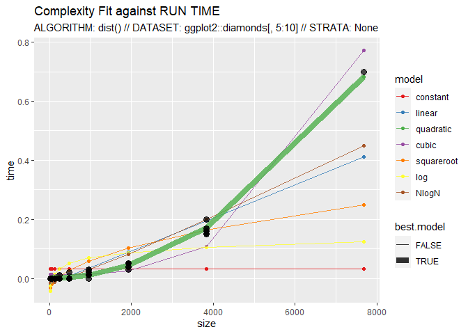
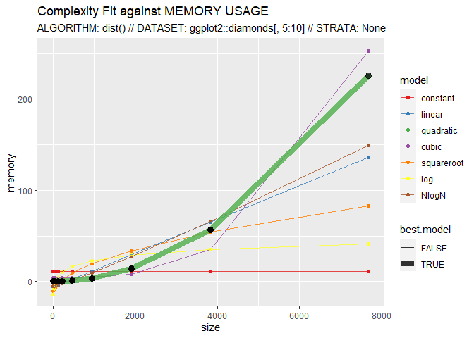
The plot output helps to compare the fit of each complexity function to the data.
Note on the memory complexity: memory analysis relies on the memory.size() function to estimate the trend and this function only works on Windows machines. If another OS is detected, the algorithm will skip the memory part.
Imports
GuessCompx requires the following CRAN packages to be installed: dplyr, reshape2, lubridate, ggplot2, boot
Installation
The package will be submitted to CRAN and hopefully available there soon. Meanwhile, you can install the beta version of GuessCompx from Github:
library(GuessCompx)

## Warning: pakke 'GuessCompx' blev bygget under R version 4.1.3

#?CompEst
Example
Here, CompEst() is used to show the quadratic complexity of the dist() function:
CompEst(d = ggplot2::diamonds[, 5:10], f = dist, replicates = 10, max.time = 10)


## $sample.sizes
##   [1]    15    15    15    15    15    15    15    15    15    15    30    30
##  [13]    30    30    30    30    30    30    30    30    60    60    60    60
##  [25]    60    60    60    60    60    60   120   120   120   120   120   120
##  [37]   120   120   120   120   240   240   240   240   240   240   240   240
##  [49]   240   240   480   480   480   480   480   480   480   480   480   480
##  [61]   960   960   960   960   960   960   960   960   960   960  1920  1920
##  [73]  1920  1920  1920  1920  1920  1920  1920  1920  3840  3840  3840  3840
##  [85]  3840  3840  3840  3840  3840  3840  7680  7680  7680  7680  7680  7680
##  [97]  7680  7680  7680  7680 15360 15360 15360 15360 15360 15360 15360 15360
## [109] 15360 15360 30720 30720 30720 30720 30720 30720 30720 30720 30720 30720
## [121] 53940 53940 53940 53940 53940 53940 53940 53940 53940 53940
##
## $`TIME COMPLEXITY RESULTS`
## $`TIME COMPLEXITY RESULTS`$best.model
## [1] "QUADRATIC"
##
## $`TIME COMPLEXITY RESULTS`$computation.time.on.full.dataset
## [1] "33.67S"
##
## $`TIME COMPLEXITY RESULTS`$p.value.model.significance
## [1] 1.731579e-96
##
##
## $`MEMORY COMPLEXITY RESULTS`
## $`MEMORY COMPLEXITY RESULTS`$best.model
## [1] "QUADRATIC"
##
## $`MEMORY COMPLEXITY RESULTS`$memory.usage.on.full.dataset
## [1] "11121 Mb"
##
## $`MEMORY COMPLEXITY RESULTS`$system.memory.limit
## [1] "16129 Mb"
##
## $`MEMORY COMPLEXITY RESULTS`$p.value.model.significance
## [1] 3.342042e-259
